📊 Exploring the Google Sheets QUERY Function Step by Step

B4ALLB4U · Oct 19, 2024

Dear All,
In today’s data-driven world, the ability to extract meaningful insights from information is crucial. Google Sheets offers a powerful tool to achieve this: the QUERY function. This function allows users to manipulate and analyze data similarly to SQL, making it accessible even for those without a background in database management.

What is the Google Sheets QUERY Function?

The QUERY function in Google Sheets enables users to retrieve data based on specific criteria and, if needed, modify formatting, perform additional calculations, change the order of columns, and more. This means your original data source remains unchanged while your working sheet displays only the columns and rows you need to complete your tasks.

Google Sheets QUERY Formula Syntax

To kick things off, let’s look at the syntax of the Google Sheets QUERY function:

!=QUERY(data, query, [headers])

data: A range of cells that you want Google Sheets to query.
query: A string containing the query written in Google API Query Language. Remember to wrap your query in double quotation marks, like this: =QUERY('data from Airtable'!A:L, "SELECT *"). Alternatively, you can refer to a cell containing the query.
headers: An optional argument to specify the number of header rows in your data set.

Google Sheets QUERY Clauses

In SQL, a clause is a component of a statement that specifies a particular action. The Google API Query Language includes nine clauses, each serving a unique purpose. These clauses are optional, meaning you don't have to include all of them in one query.

A single query string can contain several space-separated clauses, which should be written in the following order:

I’ll be explaining each query string in detail and providing a Google Sheets spreadsheet to demonstrate how it works.

Stay tuned as we dive deeper into each component of the QUERY function!

B4ALLB4U · Oct 19, 2024

1: Google Sheets Query: SELECT

The SELECT clause allows defining the columns you want to fetch and the order in which you want to organize them in your new worksheet. If the order is not specified, the data will be returned “as is” in a source spreadsheet.

One can use column IDs (the letters located at the top of every column in a spreadsheet), for example, SELECT A, B, or reference columns as Col1, Col2 and so on in the numerical sequence. You can also reference the results of arithmetic operators, scalar or aggregation functions as elements to order in this clause.

Note: if you are planning to embed Query into more complex formulas, we recommend referencing columns Col1, Col2, and so on in the numerical sequence. If you choose this option, then the data argument from the general Query syntax has to be enclosed in curly brackets.

= QUERY({data}, query, [headers])
Google Sheets Query SELECT all example
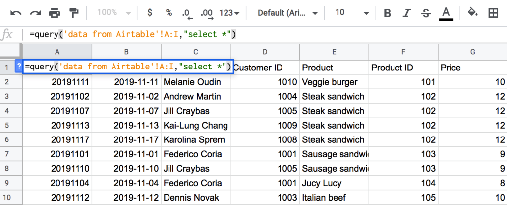
=query('data from Airtable'!A:L,"select *")

'data from Airtable'!A:L – the data range to query on
"select *" – select all information in the above-mentioned data set

Note The headers parameter allows you to specify the number of header rows to return. If you omit the header element, the returned data will include the heading row. To remove the headers, type “0” in your Query formula like this:

=query('data from Airtable'!A:I,"select *", 0)

Google Sheets Query SELECT one or multiple columns example

If a user wants to fetch only a certain or multiple columns, one needs to define them by a column ID like as follows:
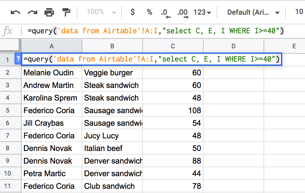
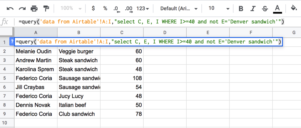
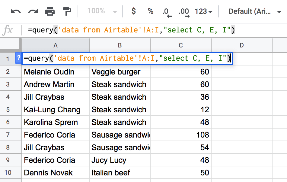
=query('data from Airtable'!A:L,"select C, E, I")

'data from Airtable'!A:L – the data range to query on
"select C, E, I" – pull all data from the columns C, E, I

Google Sheets Query SELECT multiple sheets example

If you need to query different sheets in Google Sheets, meaning that you want to select data from several different tabs of a spreadsheet, then feel free to use the below example:
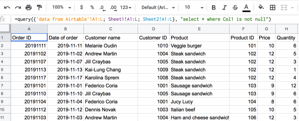
=query({'data from Airtable'!A1:L; Sheet1!A1:L; Sheet2!A1:L}, "select * where Col1 is not null")

{'data from Airtable'!A1:L; Sheet1!A1:L; Sheet2!A1:L} – an array formula enclosed into curly brackets which includes the list of sheets I want to pull data from, separated by semicolons.
"select * where Col1 is not null" – pull all data where the contents of the rows in column 1 (column A, Order ID) are not empty. Continue reading this article to learn more about the Where clause, as well as “is null” and “is not null” operators.

B4ALLB4U · Oct 23, 2024

2: Google Sheets Query WHERE

Users apply WHERE when they need to pull specific rows from the columns, they have already identified in the SELECT clause, which satisfies one or more conditions.

To compare values across rows, one needs to be aware of these basic logical operators that accompany the WHERE clause.

Google Sheets Query WHERE basic operators example

In my case, the ready-to-use formula will read:
=query('data from Airtable'!A:L,"select C, E, I WHERE I>=40")

'data from Airtable'!A:L – the data range to query on
"select C, E, I WHERE I>=40" – pull the data from columns C, E, I, where the value in column I (total price) is more than or equals 40.

Note: if you want to say that the cell is empty or its contents equal 0 – use the is null operator, and if you want to select rows that are not empty, then enter is not null.

One can combine several conditions using and, or, and not as part of the WHERE clause in the query like this:
=query('data from Airtable'!A:L,"select C, E, I WHERE I>=40 and not E='Denver sandwich'")

'data from Airtable'!A:L – the data range to query on
"select C, E, I WHERE I>=40 and not E='Denver sandwich'" – pull the data from columns C, E, I, where the value in column I (total price) is more than or equals 40 and where the string in column E (product) does not include the Denver sandwich.

Google Sheets Query WHERE advanced operators example

Use these advanced comparison operators to run more complex queries:

Here is the sample formula
=query('data from Airtable'!A:L,"select C, E, I WHERE E starts with 'C' and C like 'K%'")
'data from Airtable'!A:L – the data range to query on
"select C, E, I WHERE E starts with 'C' and C like 'K%'" – the string pulls the data from columns C, E, I, where the value in column E (product) starts with the “C” letter and where the string in column C (customer name) starts with the “K” letter.

Google Sheets Query Matches example

The matches operator helps in advanced pattern matching using regular expressions and use complex search criteria within queries.
=query('data from Airtable'!A:L,"select C, E, I WHERE E matches 'Steak sandwich'")
'data from Airtable'!A:I – the data range to query on
"SELECT C, E, I WHERE E MATCHES 'Steak sandwich'" – filters the dataset to return only the rows where column E (product) exactly matches the phrase “Steak sandwich”. It then displays the C (customer name), E (product), and I (total price) columns for those filtered rows.

B4ALLB4U · Oct 24, 2024

3: Google Sheets Query GROUP BY

This GROUP BY clause is used to group values across the selected data range by a certain condition.

Note: the columns that you mention in the SELECT clause must be present in either the GROUP BY clause or as part of the aggregation function (e.g. avg, count, max, min, sum).

Example of GROUP BY one column: Google Sheets Query SUM

Sample Dataset Query

=query('data from Airtable'!A:L,"select C, sum(I) Group by C")

'data from Airtable'!A:L – the data range to query on
"SELECT C, SUM(I) Group by C" – the string sums purchases (column I) and groups them by customer names (column C).

Example of Google Sheets Query GROUP BY multiple columns

Sample Google Sheets Query GROUP By multiple columns formula:

=query('data from Airtable'!A:L,"select C, H, sum(I) Group by C,H")

'data from Airtable'!A:L – the data range to query on
"SELECT C, H, SUM(I) Group by C,H" – the string pulls the data from columns C and H, sums purchases (column I), and groups data by customer names (column C).

Note: when using this formula, specify all columns that you defined in the Select clause in the Group by clause as well. The output will be grouped by the first column ID mentioned in the Group by clause.

B4ALLB4U · Oct 26, 2024

4: Google Sheets Query PIVOT

The Google Sheets QUERY function with PIVOT is a powerful tool for dynamically reshaping and analyzing your data without the need for manual pivot tables. It allows you to summarize data by categories (dimensions) while aggregating numerical data (metrics), all within a formula. Here's a detailed overview to help you get started:

Purpose of Using QUERY with PIVOT
• Data Summarization: Quickly condense large datasets by organizing data based on specified categories.
• Real-Time Updates: Formulas update dynamically as the data changes, which is useful for live dashboards or regularly updated sheets.
• Customizable Views: You can add filters, sorting, and specific aggregations, creating a highly customized summary table.
Syntax
=QUERY(data, "SELECT columns PIVOT column_to_pivot [aggregation function]", [headers])
• data: The cell range containing the data.
• columns: Columns to select and display in the output.
• column_to_pivot: The column with values you want to transform into column headers.
• aggregation function: Functions like SUM, COUNT, AVG, MIN, MAX, etc., which summarize data.
Benefits of Using PIVOT with QUERY
• Flexible Filtering and Sorting: More flexibility in applying filters and sorting compared to static pivot tables.
• Direct Integration with Other Functions: You can use QUERY results with other functions like ARRAYFORMULA or IMPORTRANGE for more complex reporting.
• Efficient Data Management: Enables efficient handling of large datasets, making it easier to get a summarized view without creating additional pivot tables.
Tips for Effective Use
• Always specify clear column names in your SELECT statement to avoid ambiguity.
• Experiment with multiple aggregations to get insights from different perspectives.
• Use the LIMIT clause to restrict the output if you need a quick overview without overwhelming details.

Using the PIVOT clause one can convert rows into columns, and vice versa, as well as aggregate, transform, and group data by any field.

Note: the columns that you mention in the SELECT clause must be present in either the GROUP BY clause or as part of the aggregation function (e.g. avg, count, max, min, sum).

Google Sheets Query PIVOT without GROUP BY example

=query('data from Airtable'!A:L,"select sum(G) Pivot E")

'data from Airtable'!A:L – the data range to query on
"SELECT SUM(G) Pivot E" – the string sums the prices of all burgers sold (column G) and groups them by the product (column E).

Sample Dataset : Google sheet

Google Sheets Query PIVOT with GROUP BY example

=query('data from Airtable'!A:L,"select C, sum(G) Group BY C Pivot E",1)

'data from Airtable'!A:L – the data range to query on
"SELECT C, SUM(G) Group BY C Pivot E" – the string returns a PIVOT table which has the names of burgers (column E) in the heading row, and the list of customers (column C) as the main column, showing which burgers customers bought and how much they paid (column G).

B4ALLB4U · Oct 27, 2024

Google Sheets Query ORDER BY (ascending or descending)

The ORDER BY clause in Google Sheets' QUERY function allows you to sort data in either ascending or descending order based on one or more columns. Here’s how you can use it effectively:

Basic Syntax of QUERY with ORDER BY
=QUERY(data, "SELECT column_list ORDER BY column [ASC|DESC]")

data: Range of cells containing the data you want to query.
column_list: Columns to be retrieved (e.g., A, B, C). Use * to select all columns.
column: The column to sort by (e.g., A, B).
ASC: Sorts the data in ascending order.
DESC: Sorts the data in descending order.

Example of Google Sheets Query ORDER BY to sort in ascending order

=query('data from Airtable'!A:L,"select * where A is not null order by A")

'data from Airtable'!A:L – the data range to query on
"SELECT * WHERE A IS NOT NULL ORDER BY A" – the string pulls all data and orders it by order ID (column A) in ascending order.

Example of Google Sheets Query ORDER BY to sort in descending order

=query('data from Airtable'!A:I=L,"select * order by A DESC")

'data from Airtable'!A:L – the data range to query on
"SELECT * ORDER BY A DESC" – the string pulls all data and orders it by order ID (column A) in descending order.

Example of Google Sheets Query Sort By Date

To sort the data by date, you can use the ORDER BY clause followed by date.
=QUERY('data from Airtable'!A1:L21,"ORDER BY B",1)

'data from Airtable'!A:I – the query data range
"ORDER BY B" – the string to sort the entire dataset based on the values in column B (date of order) in ascending order.

B4ALLB4U · Nov 2, 2024

Google Sheets Query LIMIT (+ formula example)

In Google Sheets, the QUERY function can be combined with the LIMIT clause to control the number of rows returned in your results. Here’s the basic syntax and an example for using LIMIT with the QUERY function:

The ready-to-use formula
=query('data from Airtable'!A:L,"select * Limit 5")

'data from Airtable'!A:L – the data range to query on
“SELECT * Limit 5" – the string pulls all data and limits the returned result to the first 5 rows + the header.

B4ALLB4U · Nov 10, 2024

Google Sheets Query OFFSET

Using this clause you may ask Google Sheets to skip a pre-defined number of rows from the top of your data source spreadsheet.
Google Sheets Query OFFSET only formula example
=query('data from Airtable'!A:L,"select * Offset 10")

'data from Airtable'!A:L – the data range to query on
"SELECT * OFFSET 10" – the string pulls all data and skips the first 10 rows excluding the header.

Google Sheets Query OFFSET accompanied by LIMIT example

If OFFSET is combined with the LIMIT clause, though it follows LIMIT in the syntax, it will apply first.
=query('data from Airtable'!A:L,"select * Limit 5 Offset 10")

'data from Airtable'!A:L – the data range to query on
"SELECT * LIMIT 5 OfFSET 10" – the string pulls all data, skips the first 10 rows, and limits the result to 5 rows excluding the header.

B4ALLB4U · Nov 14, 2024

Google Sheets Query LABEL

The LABEL clause allows you to assign a name to a heading field of one or multiple columns. However, you won’t be able to apply it instead of a column ID in a query string.

One can use column IDs or the results of arithmetic operators, scalar, or aggregation functions as elements in this clause.
=query('data from Airtable'!A:L,"select * label C 'customer', E 'Burger', I 'Total paid'")

'data from Airtable'!A:L – the data range to query on
"SELECT * LABEL C 'customer', E 'Burger', I 'Total paid'" – the string pulls all data, and gives columns C, E and I new labels.

B4ALLB4U · Nov 22, 2024

9: Google Sheets Query FORMAT

Users apply the FORMAT clause to format NUMBER, DATE, TIME, TIMEOFDATE, and DATETIME values for one or multiple columns.

Example of FORMAT clause: Google Sheet Query Date

=query('data from Airtable'!A:L,"select B, G, I, J label J 'Hour' format B 'dd-mmm-yyyy', G '##.00', I '##.000', J 'HH'")
'data from Airtable'!A:L – the data range to query on
"SELECT B, G, I, J label J 'Hour' format B 'dd-mmm-yyyy', G '##.00', I '##.000', J 'HH'" – the string pulls the data from columns B, G, I, and J, formats the date in the B column, the number in the G and I columns, and the time in the J column, also changing its label to ‘Hours’.

B4ALLB4U · Dec 26, 2024

Dear Friends.!

Prefer to watch and learn? Check out in-depth video on mastering the Google Sheets QUERY function. This video complements the tips and tricks in this guide, offering a visual approach to efficient data management. Get started now and streamline your data tasks!

Get Your Spreadsheet Work Done with Our QUERY Template!
Simplify data analysis, filter results easily, and explore advanced scenarios – all in one convenient Template.